Descriptive and Inferential Statistics

Math Tip!!!

Descriptive statistics are numbers that are used to summarize and describe data. The word "data" refers to the information that has been collected from an experiment, a survey, a historical record, etc. If we are analyzing birth certificates, for example, a descriptive statistic might be the percentage of certificates issued in New York State, or the average age of the mother. Any other number we choose to compute also counts as a descriptive statistic for the data from which the statistic is computed.

Several descriptive statistics are often used at one time, to give a full picture of the data. We decide which descriptive statistic is appropriate based on the shape of the curve and/or the nature of the distribution.

 

Measures of Central Tendency

 

With tables and graphs we have a picture of the distribution of our data. Now we will look at some numerical ways to summarize them. The key to summarizing you data lies with the central tendency. A measure of central tendency is a calculated value that is typical of the entire distribution. There are three primary measures of central tendency:

 

A. Mean =

• The arithmetic average of all scores
• Add all scores and divide by the total number of scores in the group.

 

 

• The mean is pulled towards the high or low end of the distribution by outliers
• Results in a skewed distribution
• The mean is the statistic on which most calculated significance tests are based.
• Appropriate for ratio or interval data but not nominal and ordinal scaled data.

Example 1:

Data point	X
1	10
2	11
3	15
4	12
5	16
N = 5	∑x = 64

 

 

---

PRACTICE PROBLEM 1.3:

Find the mean of the following data set

 

9, 8, 3, 7, 9, 7, 9, 5, 8, 5, 4, 6, 6, 7, 5, 3, 2, 8, 5, 8, 8, 8, 4

 

ANSWER 1.3 (Mouse-Over to Check Your Answer).

 

---

 B. Median =

• Point or position in a distribution that divides the scores in two equal parts; the midpoint or middle score

From the low value, count this many places to find the Mdn value.

 

• Calculating the median
• First, put all distribution scores in order from low to high.
• If the data set is odd numbered then simply find the middle score using the count value above.
• If the data set is even numbered then find the middle two numbers using the count value above and take their average.
• This average is your median.
• Note that when the data set is even numbered, the median does not necessarily represent a value that is in the distribution.
• Characteristics:
• The median is appropriate for ratio, interval, or ordinal data, but not nominal.
• The median is resistant to (not affected by) outliers.

Example 2:

Data point	x
1	10
2	11
3	12
4	15
5	16
N = 5	∑x = 64

Example 3:

Data point	x
1	10
2	11
3	12
4	15
5	16
6	17
N = 5	∑x = 64

 

---

PRACTICE PROBLEM 1.4:

Find the Median of the following data set.

 

9, 8, 3, 7, 9, 7, 9, 5, 8, 5, 4, 6, 6, 7, 5, 3, 2, 8, 5, 8, 8, 8, 4

 

ANSWER 1.4:

 

---

 

C. Mode =

• The most frequently appearing score(s) in a distribution
• There may be more than one (making a bimodal distribution).
• Characteristics:
• The mode is appropriate for ordinal and nominal data.
• It is easier to find the mode if the distribution is in order from low to high.

 

 

---

 

PRACTICE PROBLEM 1.5:

Find the Mode of the following data set

 

9, 8, 3, 7, 9, 7, 9, 5, 8, 5, 4, 6, 6, 7, 5, 3, 2, 8, 5, 8, 8, 8, 4

 

ANSWER 1.5:

 

---

Measures of Variability

 

What is variability?  Variability is a measure of dispersion; the degree to which individual scores in a data set differ from one another.  It is another set of descriptive statistics. 

 

A.  Range =

• The most simplistic measure of variability
• The highest score in a data set minus the lowest score
• It gives you a rough idea of what your data looks like. 
• A large range means there is more variability.
• A small range means there is less variability.

Example 4:

Exam scores for two different courses:

 

Class A	Class B
78	82
82	90
95	91
100	79
65	78
= 84	= 84
= 35	= 13

 

 

• Which class will be more challenging to teach?
• Why?
• How would knowledge of the range change our teaching style?

The challenge with range

 

B. Standard Deviation

 

1. Population Standard Deviation = or

• The most widely used measure of variability is the standard deviation
• A calculated number that represents the average distance between the mean and the observed scores
• or represents the population standard deviation
• We use this value when it is the given value for the populations standard deviation, or when ALL scores in a population are known allowing us to calculate the populations standard deviation.
• Calculating

 1) Set up the following table and take the sum of all raw scores (∑X).

 

Data point	X
1	10
2	11
3	12
4	15
5	16
6	20
7	13
8	15
9	17
10	19
N = 10	∑x = 148

 

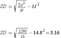
2) Add another column made of the square of each X, taking the sum of this column (∑X²).

 

Data point	X	X2
1	10	100
2	11	121
3	12	144
4	15	225
5	16	256
6	20	400
7	13	169
8	15	225
9	17	289
10	19	361
N = 10	∑x = 148	∑x2 = 2290

 

3) Find the Mean.

 

4) Use the collected sum'd data in the formula:

 

 

 

---

 

PRACTICE PROBLEM 1.6:

The following data set represents a population of scores. Find the SD.

 

10, 6, 11, 15, 18, 20, 17, 12, 10, 9, 19, 16, 14, 11, 10, 21, 22

 

ANSWER 1.6:

 

---

 

2. Estimated Standard Deviation =

• It is used with samples to estimate parameters in a population.
• S will be the statistic we use most often throughout this course.
• Goes back to Samples vs. Populations
• The purpose of statistical analysis is to compare a sample to a population, or samples to other samples.
• Either way, if samples estimate the population, then we need an estimate of the samples standard deviation
• Bottom line: When it's a sample, use the following formula for standard deviation
• Calculating

 

NOTE the differences between and

 

 1) Set up the following table and take the sum of all raw scores (∑X)

 

Data point	X
1	10
2	11
3	12
4	15
5	16
6	20
7	13
8	15
9	17
10	19
N = 10	∑x = 148

 

2) Add another column made of the square of each X, taking the sum of this column (∑X²)

 

Data point	X	X2
1	10	100
2	11	121
3	12	144
4	15	225
5	16	256
6	20	400
7	13	169
8	15	225
9	17	289
10	19	361
N = 10	∑x = 148	∑x2 = 2290

 

3) Use the collected sum'd data in the formula:

 

 

---

PRACTICE PROBLEM 1.7:

The following data set represents a sample of scores. Find the S

 

10, 6, 11, 15, 18, 20, 17, 12, 10, 9, 19, 16, 14, 11, 10, 21, 22

 

ANSWER 1.7:

 

---

 

3. Variance =

• Variance is another descriptive statistic that is also a measure of variability.
• Variance is the square of standard deviation, therefore does not have a practical interpretation in terms of data. However it is commonly used in more statistics.
• Calculation: Find S, then square it.

 

---

PRACTICE PROBLEM 1.8:

The following data set represents a sample of scores. Find the S²

 

10, 6, 11, 15, 18, 20, 17, 12, 10, 9, 19, 16, 14, 11, 10, 21, 22

 

ANSWER 1.8:

 

---

 Take a moment to compare the three formulas. Make sure you understand the difference among the 3.

  

Descriptive statistics are just descriptive.They do not involve generalizing beyond the data at hand. Generalizing from our data to another set of cases is the business of inferential statistics.

It is not practical to ask every single American how he or she feels about the fairness of the voting procedures. Instead, we query a relatively small number of Americans, the sample, and draw inferences about the entire country, the population, from their responses. The Americans actually queried constitute our sample of the larger population of all Americans. This is inferential statistics.

Since we are inferring the characteristics of a large body of possible observations from a smaller select group of observations, it is crucial that it be representative. In looking at our sample of Americans, for it to be representative, it must not over represent one kind of citizen at the expense of others. For example, something would be wrong with our sample if it happened to be made up entirely of Florida residents. If the sample held only Floridians, it could not be used to infer the attitudes of other Americans. The same problem would arise if the sample were comprised only of Republicans. Inferential statistics are based on the assumption that sampling is random. We trust a random sample to represent different segments of society in close approximation to the actual population proportions.

 

return to top | previous page | next page