Describing the Shape of Distributions

The concept of the distribution was introduced at the beginning of this module. We have since covered the concepts of central tendency and variability as well as frequency charts and graphs. Let's end by using these concepts to describe the shape of a distribution.

 

The shape of the distribution cannot be ignored as it tells us which of the descriptive statistics we should be using. Though we have three measures of central tendency, they are not all appropriate for all situations.

 

Common distribution shapes are listed here:

 

A. Symmetric distributions

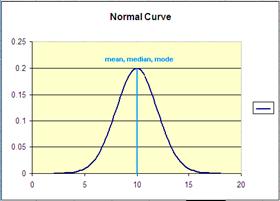
• The Normal bell-shaped distribution is probably the most well-known symmetric distribution.
• Scores that fall far from the mean are less frequent and fall on both sides of the mean (-/+).
• Measures of central tendency are all equal.
• This is, in fact, where the term central tendency comes from.
• All measures of central tendency will fall on the midline, the central point.
• Ex. normal distribution or normal curve.
• It is most appropriate to report the mean for such a distribution.

 

 

B. Skewed distributions

• When scores with highest frequency do not fall close to the mean
• Skewed distributions can be:
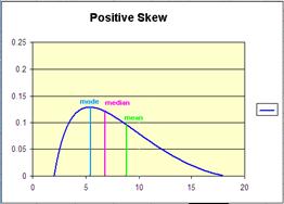
• Positively skewed - most frequent scores are low; tail is toward the high scores
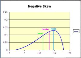
• Negatively skewed - most frequent scores are high; tail is toward low scores
• You can detect skew by looking at the values of central tendency.
• In a skewed distribution, the central tendency will not be equal.
• moving up the tail, you will typically pass the mean, then median, finally the mode.
• So: if Mode < Median < Mean = Positive Skew, most typical
• But: if Mode > Median > Mean = Negative Skew, most typical

 

 

• It is most appropriate to report the median for such a distribution.
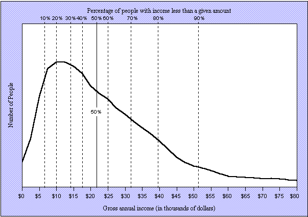
• Why? Think of an income distribution. The most unfortunate example of a positive Skew.
• Most individuals in a population may earn $12,000 / year.
• A few individuals in the same population may earn $80,000 / year.
• In this case we would report the median income because the mean would be much higher than $12,000/year.
•  Remember: The median is not affected by outliers.

 

C. Bimodal distributions

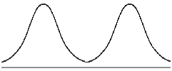
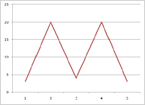
• When graphed it has two humps:

 

 

• Each hump is caused by a mode.
• When does this happen?
• Consider the graph below represents attitudes towards owning handguns among 50 respondents.
• If the categories represent a 5 point scale, with 1 being strongly disagree and 5 being strongly agree and 3 being unsure, then this data would suggest an equal number of people moderately agreeing and moderately disagreeing.
• It is most appropriate to report the modes for such a distribution.
• Why? Both the mean and the median would fall around 3.This would suggest that most people were unsure.That is clearly not the case and would not be accurate.

 

 

 

 

D. Kurtosis

• Describes the 'peakedness' in a curve and the thickness of the tails
• Occurs in normally distributed data sets (Bell curves)
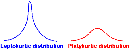
• Leptokurtic
• Tall and skinny compared to the Normal bell curve with an excess of extreme values causing the tails to be thicker than the Normal bell curve
• kurtosis value > 0
• Platykurtic
• Short and fat compared to the Normal bell curve with fewer extreme values causing the tails to be thinner than the Normal bell curve
• kurtosis value < 0
• Mesokurtic
• The Normal bell curve is a common example.
• kurtosis value = 0
• Does not affect the central tendency.

 

 

 

• A rule of thumb you can use to determine the type of kurtosis by comparing the standard deviation to 1/6 of the Range

 

---

PRACTICE PROBLEM 1.9:

Describe the data set from practice problem #1 and 2.

  

ANSWER 1.9

 

return to top | previous page | next page