Pearson Product-Moment Correlation Coefficient

Let's look at how we can calculate the correlation coefficient using the method developed by Karl Pearson during the latter half of the nineteenth century while conducting a series of studies on individual differences with Sir Francis Galton. Pearson called his equation the product moment correlation coefficient. We typically now refer to it as the Pearson's r. The calculation is based on the concept of the Z scores; specifically, taking the mean of the Z score products from the X and Y variables.

The formula for Pearson's r is:

 

You can see in the numerator involves finding the Z scores for each of the x and y coordinates, multiplying those Z scores together, and finally adding them all up. And then you get to divide by n – 1 ! This can quickly become a labor-intensive project, so instead we will use a form that cuts down on the computational labor:

One further note – Generally the two variables play specific roles in a bivariate study. One variable, x, is the independent variable, while y is the dependent variable (more on this in the next lesson). However, when computing Pearson's r, these roles do not matter. You will get the same correlation value even if you reverse the two variables.

 

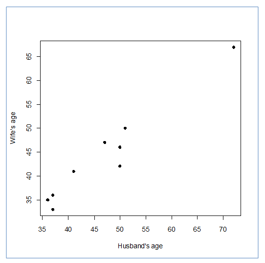
By way of our first illustration, let's consider something with which we are all familiar: age. Let's begin by asking if people tend to marry other people of about the same age. Our experience tells us "yes," but are we confident with this answer (Notice I didn't say "sure")? One way to address the question is to look at pairs of ages for a sample of married couples. The samples date below does just that with the ages of 10 married couples. Going across the columns we see that, yes, husbands and wives tend to be of about the same age, with men having a tendency to be slightly older than their wives. This is no big surprise, but at least the data bear out our experiences, which is not always the case. What we know of statistics, however, tells us that what we see is not always significant. So lets apply the Pearson r formula and see what happens.

 

Husband (x)	36	72	37	36	51	50	47	50	37	41
Wife (y)	35	67	33	35	50	46	47	42	36	41

 

Always start an investigation of bivariate data with a graph. Notice the scatterplot indicates a fairly strong, linear association between the ages of husbands and wives.

If you look at the formula for a minute you will notice that it is all old material with one exception. We now have an additional column of information that we need to sum. XY. There's nothing to it! Look at the following table.

 

	Husbands		Wives
Pair	X	X2	Y	Y2	XY
1	36	1296	35	1225	1260
2	72	5184	67	4489	4824
3	37	1369	33	1089	1221
4	36	1296	35	1225	1260
5	51	2601	50	2500	2550
6	50	2500	46	2116	2300
7	47	2209	47	2209	2209
8	50	2500	42	1764	2100
9	37	1369	36	1296	1332
10	41	1681	41	1681	1681
∑ =	457	22005	432	19594	20737

 

XY is simply the product of columns X and Y. Therefore, 36 x 35 = 1260. Therefore, 36 x 35 = 1260, 72 x 67 = 4824, and so on.

Another issue to consider is how many data points we have. Although we have 10 for husbands and 10 for wives, we do not have 20 independent data points. Instead, we have 10 pairs of data points, so n = 10. Remember, correlation concerns the relationship between the two variables, and husbands and wives definitely form pairs. It certainly wouldn't make sense to treat all 20 individuals as independent and allow them to pair up in some random manner!

N = # pairs

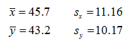
So with the above information we can calculate the Sx (S for the X column) and the Sy (S for the Y column) and we are ready to go. Since you have had plenty of practice so far, do that now. Find the mean and the standard deviations of x and y, you should find:

 

Did you have problems with either Sx or Sy? If so, your work should have looked like this

 

Now just plug it all into the formula!

  

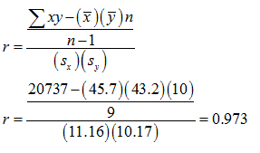
So based on our data, there is a positive correlation of 0.974 between the ages of husbands and wives. Now, is this significant? To check for a significant Pearson r correlation, we turn to a new set of tables. The concept, however, will remain the same. We need to compare our calculated r to a critical r value found in the table

A hypothesis test for correlation will start with a null hypothesis of "zero correlation." Then the alternative hypothesis will be "there is a non-zero correlation." In the hypotheses below, the Greek letter rho represents the true correlation in the population from which our sample is drawn.

 

Critical values for the Pearson r

Df = N-2	α = 0.05	α = 0.01
1	0.99700	0.99990
2	0.95000	0.99000
3	0.87800	0.95900
4	0.81100	0.91700
5	0.75400	0.87400
6	0.70700	0.83400
7	0.66600	0.79800
8	0.63200	0.76500
9	0.60200	0.73500
10	0.57600	0.70800
11	0.55300	0.68400
12	0.53200	0.66100
13	0.51400	0.64100
14	0.49700	0.62300
15	0.48200	0.60600
16	0.46800	0.59000
17	0.45600	0.57500
18	0.44400	0.56100
19	0.43300	0.54900
20	0.42300	0.53700
21	0.41300	0.52600
22	0.40400	0.51500
23	0.39600	0.50500
24	0.38800	0.49600
25	0.38100	0.48700
26	0.37400	0.47900
27	0.36700	0.47100
28	0.36100	0.46300
29	0.35500	0.45600
30	0.34900	0.44900
35	0.32500	0.41800
40	0.30400	0.39300
45	0.28800	0.37200
50	0.27300	0.35400
60	0.25000	0.32500
70	0.23200	0.30300
80	0.21700	0.28300
90	0.20500	0.26700
100	0.19500	0.25400

 

For a Pearson r correlation, our df = N - 2, where N is still equal to the number of pairs. So what is our decision? Even if we use the more conservative alpha = 0.01, our calculated r (0.974) exceeds the critical r (from the table) of 0.765. So our correlation is significant.

 

When it comes to correlations, we are faced with a problem not observed with our previous hypothesis testing. The issue is with significance. Look at the above table. If we had 3 subjects, what is the critical r? With alpha = 0.05 and a df=1 our critical r would be 0.997. That means that we would need a very strong correlation for significance. Now look at the other end. What if we had a df=100? Now our critical r becomes 0.195 at alpha = 0.05. What this may tell you is that all we need for a significant correlation is a high number of subject pairs! This means that if the data set is large enough, even a very slight correlation may appear to be significant. You should always examine a scatterplot of your data before you considering computing and testing correlation. If the scatterplot doesn't suggest a linear pattern in the data – don't calculate correlation!

 

Another statistic of interest is called the coefficient of determination (r²). Good news, that is the formula! Just square the r. The coefficient of determination is used to establish the proportion of the variability among the Y scores that can be accounted for by the variability among the X scores. For the husband and wife data we computed Pearson's r to be 0.974 (remember – this means the data points follow quite closely to a positive-sloping line). If we now square r we get approximately 0.949. As the coefficient of determination (often just called r-squared by statisticians) we generally report this number in percent form, so we have about 95%.

We originally suspected that husbands and wives would tend to be similar in age. A scatterplot of the data suggests there is a fairly strong linear relationship present. And the correlation of 0.974 further describes how strong the relationship is (close to 1 = strong linear relationship). Now we can use r-squared to provide one more perspective on this relationship. To say the r-squared value is 95% means that of all the variation among the y values (the ages of the women), about 95% of that variation can be directly attributed to the linear relationship with the x values (the ages of the men). The remaining 5% of the variation in the ages of the women is then due to other factors besides the ages of the men.

Note that the closer to 100% the value of r-squared, the stronger the relationship between x and y. However, we cannot say that changes in x cause the variation in y. All we can say is there is a strong association between the two variables. There may be some other underlying factor that actually serves as the engine causing change. One of the most common errors made in interpreting bivariate data is to wrongly equate causation with association.

 

 

PRACTICE PROBLEM #3

For the following data set, find the Pearson r and the r².

X	Y
12	10
2	3
5	7
9	5
11	9
10	8
4	6
1	3

 

ANSWER

 

 

return to top | previous page | next page