Linear Regression and Prediction

Now on to the predictions.

In linear regression we construct a model (equation) based on our data. We can then use this model to make predictions about one variable based on particular values of the other variable. The variable we are making predictions about is called the dependent variable (also commonly referred to as: y, the response variable, or the criterion variable). The variable that we are using to make these predictions is called the independent variable (also commonly referred to as: x, the explanatory variable, or the predictor variable).

This is, in fact, the line that we were eyeballing in the opening section of the module. Using linear regression we will be able to calculate the best fitting line, called the regression line. And just what is the criterion for the best fitting line? It is simply the line that minimizes the sum of our square errors which is the sum of the differences between the plotted points and our line as illustrated below.

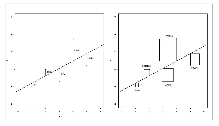
Why complicate things with all of this talk of squaring errors? And what are errors, anyway? Remember, that to a statistician, an error refers to variation, not a mistake. The difference between the actual value of y and the value of y predicted by the model is called a residual – a type of error. In the diagram below on the left, these residuals are drawn on a scatterplot as vertical line segments. You might think that the linear regression line would be the best fitting line that would minimize these errors. However, the mathematical process of minimizing involves adding up the quantities to be minimized, which in this case (and all linear regression) the sum of the residuals is zero. This is because some of the residuals are positive and some are negative and they all end up canceling each other out.

One way to keep the negative residuals from canceling out the positive residuals is to square all of the residuals. Since squaring will always produce a positive number, the sum of these squared residuals will be non-zero. The scatterplot below on the right shows these squares.

 

The formula for a regression line is

 

Where:

b = slope

a = intercept

The symbol over y is called a "hat" so the term is literally called "y-hat" and indicates that this equation produces estimated (or predicted) values of the dependent variable and not the actual data values.

You might have also noticed the order of the two terms on the right are reversed from how you might have seen the equation of a linear function in a high school algebra class. Technically, the order of two terms that are added is irrelevant as the answer is the same either way. Statisticians generally prefer the order shown above because they are quite often dealing with more than one predictor variable (more than one "x") and this arrangement always places the intercept term first, followed by as many predictor variables as necessary.

 

To calculate the regression line we will need the slope and the intercept. First, the slope.

The slope of a line describes the rate of change in y for every unit change in x. In other words, when x increases by 1, y increases (or decreases if negative) by "b." You may remember hearing "rise over run" over and over again in your early math classes. Or, maybe you have blocked it out. The good news is that we are returning to that same concept here for the calculation of the slope.

Simply stated, this means to find the slope of our line we would count up along the y axis and divide that value by the value going across the x axis. Of course it isn't that easy but it's close.

Second, the intercept. The intercept is the point at which the line crosses the ordinate (Y axis). After we have the slope we can find the intercept.

 

Let's try this out using our last example. If you remember, our data was based on the ages of wives and husbands.

Husband (x)	36	72	37	36	51	50	47	50	37	41
Wife (y)	35	67	33	35	50	46	47	42	36	41

With:

  

Now the predictions are simple. If we want to predict a value of y, we just enter a value of x. Try it with the data we have. If we know a husband's age is 36, (1) what would we predict the wife's age to be? (2) What if the husbands age is 51? You should have predicted (1) and (2).

Were they close to the actual data we collected? If not, remember that our correlation was 0.97 (97%) and not 1.0 (100%)!

The relationship between the two variables (husband's age and wife's age) is described by the slope coefficient: "For every one-year increase in the age of the husband, our model predicts an increase in the age of the wife of about 0.888 years."

The interpretation of the intercept, as is often the case, is somewhat silly when taken literally. Since x represents the husband's age, if x was allowed to be equal to 0, the predicted y value would be 2.618. That's right - if the husband is 0 years old, the model predicts the age of the wife to be a little less than 3 years old! In reality, of course, this is nonsense. Predictions cannot be made reliably when we go outside of the range of our collected data (this sort of prediction is called "extrapolation"). Since the youngest ages in our data set are in the middle 30s, our model only reasonably applies to ages down to the middle 30s.

 

PRACTICE PROBLEM #4

Set up a regression line for practice problem #3

Predict y's for x's of 6, 8, and 10.

ANSWER

 

 

return to top | previous page | next page