Computer Generated Model

In the last couple of sections, we learned that linear regression is used to derive the actual equation of the best fitting line through the points on a scatterplot. We also learned that regression allows you to determine how well one variable can be used to predict another.

We then calculated the regression line by hand, after finding the Pearson r. Well, we don't always have to do these things by hand. In fact, there are many programs that would allow us to do any number of analyses with the aid of a computer (and not just our trusty calculator).

One such program is SPSS. SPSS is a very powerful computer software package for statistical analysis and one used on campuses around the world. Unfortunately, as with many things, with a powerful software tool comes a lot of confusion. For this final section in this module, we will run through an example using SPSS to conduct a regression analysis.

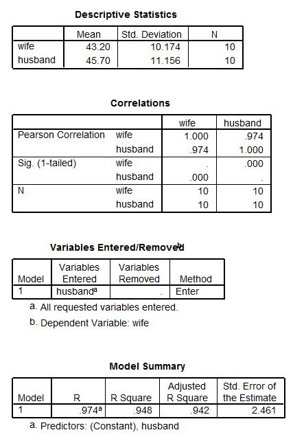
After having worked through the example on the ages of husbands and wives, here is SPSS (version 15.0) regression output for that example.

Regression

You will recognize some of the statistics in these tables from what we calculated in the previous lessons. For example, the first table gives the means and standard deviations for each variable. Another table (Model Summary) gives the values of Pearson's r and the coefficient of determination (r-squared). The Coefficients table provides the information we need to write the least squares regression equation:

The coefficients table also gives the standard error, t statistic, and significance level for hypothesis testing on the coefficients in the model. In this case, the slope (which describes the relationship between the ages of husbands and wives) has a t statistic of 12.077 and a corresponding significance level of 0.000. It's not really 0.000 - the software is programmed to only show the significance level to 3 decimal places. But it is certainly less than an alpha of 0.01 which makes the slope coefficient significant.

You will also have noticed there is much more information here. That is because the people who programmed the software did not know exactly which information we might need for this particular analysis. It is generally easier for the default output to include a wider range of information than we might actually need in a simple case than to provide less information and force the user to do extra work in order to get what is needed for more complicated analysis. Therefore it is up to us to pick and choose the relevant information.

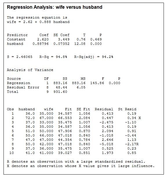
You will again notice familiar information even though the appearance is rather different. One particular difference is that the default output for Minitab actually displays the regression equation:

Notice the equation doesn't use variables x and y, but rather more descriptive names. This is common practice in statistics and can greatly aid in communicating understanding for what an equation represents.

The table at the bottom shows additional information including: the original data, the predicted (fitted) values of the dependent variable (predicted wife's age), and the residuals.

[The SPSS and Minitab output for the husband and wife data is probably sufficient for this page. However, if the existing study about workplace strength is also used, make the following minor changes.]

Minitab is another statistics software package that is available. Here is the output for the husband and wife age data from Minitab (Release 14.0):

First let's start with a little background for our example case study.

Is being physically strong still important in today's workplace? In our current high-tech world one might be inclined to think that only skills required for computer work such as reading, reasoning, abstract thinking, etc. are important for performing well in many of today's jobs. There are still, however, a number of very important jobs that require, in addition to cognitive skills, a significant amount of strength to be able to perform at a high level. Take, for example, the job of a construction worker. It takes a lot of strength to lift, position, and secure many building materials such as wood boards, metal bars, and cement blocks. In addition, the tools used in construction work are often heavy and require a lot of strength to control. When was the last time you tried to operate a jackhammer?

There are many more jobs such as electrician and auto mechanic that also require strength. An interesting applied problem that arises is how to select the best candidates from among a group of applicants for physically demanding jobs. One obvious way might be to take them to a job site and have them demonstrate that they are strong enough to do the job. Unfortunately, this approach might be too time consuming if you are having to select a large number of people from a large applicant pool. Also, you risk injury to applicants who are not strong enough to do the job. A solution to this problem is to develop a measure of physical ability that is easy and quick to administer, does not risk injury, and is related to how well a person performs the actual job. A study by Blakely, Quiñones, and Jago (1995) published in the journal Personnel Psychology reports on the research results of just such a measure. That study, and this case study, looks at methods for determining if these strength tests are related to performance on the job. The principles and methods associated with this case study also apply to any number of variables other than strength and job performance.

Below are SPSS outputs for each strength test (arm and strength) predicting each of the two performance measures (ratings and simulations). There are several numbers that are particularly noteworthy. First, the R-Squared indicates the proportion of variance in the dependent variable explained by the independent variable. Thus, for predicting Ratings from arm strength, you can see that the linear equation predicts .048 or approximately 5% of the variance in ratings. Next, the Standard Error indicates how far off you would be, on average, if you were to use the independent variable to predict scores on the dependent variable. Thus, if you used arm strength scores you could predict ratings with an average error of 8.34 (on a 60-point scale).

The specific equation for the line of best fit can be derived from the numbers under the "B" column. The first number indicates the slope of the line (.089 for the first example) and the second number indicates the intercept (33.97 for the first example). Thus, one could get a predicted Ratings score by plugging a person's arm score into the regression line equation:

Ratings = 33.97 + 0.089 (Arm)

The regression outputs for the other strength scores and performance measures are presented below.

 

Regression Equation of ARM predicting RATINGS

The last bit of information to take from our results is listed in the very last column 'sig'. This is the p-value. The p-value for this example is .0071, well below 0.05 and even 0.01. Therefore, the coefficients used to develop this regression line are significant.

return to top | previous page | next page