F ratio
Around the 1920s, Sir Ronald Fisher introduced a new analytical procedure called Analysis of Variance (ANOVA) which employs a new distribution called the F distribution. This also means a new hypothesis test using the F ratio
So far, we have only conducted analyses of two groups at one time using Z scores or t ratios. What if we have more than two groups? What if, for example we are evaluating the effectiveness of drug doses? We could use a t test to evaluate the differences in effect between 5mg and 15mg.
We may, however, also want to consider a dose of 25mg. At this point, some individuals are tempted to make the mistake of conducting multiple statistical inferences simultaneously.
For example, we could conduct a series of t tests. If we had two groups, the decision would be based on A vs. B. But with three groups (5mg, 15mg, and 25mg) we would have to base our decisions on A vs. B, B vs. C, and A vs. C. The problem is that conducting multiple statistical inferences leads to the family-wise error rate, the probability of making one or more Type I errors among all the hypotheses because with each simultaneous statistical inference our alpha inflates (becomes less conservative) making it easier to show a significant difference among ALL groups. Of course if we make a Type I error, there actually was NOT a difference. The following table illustrates the inflation effects on the alpha level. So if we were to string 10 t tests in a row, even if we were to set the alpha level at 0.05, the alpha level would ultimately be operating at an level inflated to 0.40. Meaning that the probability of committing a Type I error is 40%.
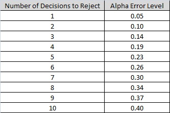
Constructed from the follow general formula, where d equals the number of decisions.
Now, back to the ANOVA, a major benefit is that the researcher can conduct comparisons of three or more groups using one inference instead of multiple inferences and thus avoiding the inflated alpha level. And instead of the mean, as with the previous analyses, we will use measurements of variance to conduct our hypothesis test. How? Well that's the fun part.
Like the t test, there are multiple forms of the ANOVA. In this module we will look at the one-way ANOVA.
One-way ANOVA
The one-way ANOVA consists of only one independent variable with three or more levels (our groups) and one dependent variable. For our example let's consider an interesting study that was once conducted with the help of the Texas Department of Public Safety. Participants were divided into three groups and each group was given a different amount of alcohol. The participants were then asked to drive an obstacle course, under supervision, and their reaction times were measured.
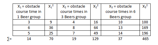
Like this old study, we are going to use amount of alcohol consumed as our IV with the three levels (1 beer, 3 beers, and 6 beers) each having only three subjects (to keep our example easy although, in reality, many more subjects are needed for a proper analysis). For this example we will use the following completely made up data consisting of times (in minutes) to complete the obstacle course.
| 1 Beer | 3 Beers | 6 Beers |
| 3 | 4 | 10 |
| 6 | 8 | 13 |
| 5 | 7 | 14 |
The researchers' question of interest is whether there is a difference in mean time to complete the obstacle course for the three different groups. If you define the true mean time for each group as  ,
,  , and
, and  respectively, the hypotheses are:
 at least one mean differs from the others
It is worth noting that the means referred to in the hypotheses are not the particular means resulting from the carrying out of this study. Rather, they refer to the theoretical mean times for each treatment group regardless of which subjects eventually were randomly assigned to the groups.
Before we get started you should have an understanding of 3 symbols that may have been used previously, sometimes interchangeably, but now take on specific meaning: N, n, and K
N = The total number of observations
n = The number of observations within a group
K = The number of groups.
After we have our data we want to find the summed data ( ) just like with measures of standard deviation.
In order to determine a significant difference among these groups we need to calculate the F ratio. While the previous ratios using Mean difference only needed to be concerned with the differences between groups the F ratio, working with variance must be concerned with the variability between groups as well as the variability within groups. The F ratio therefore looks like this:
Note that the F distribution is actually family of distributions (like the t distribution) each differing with regards to degrees of freedom. We'll pick up the details as we go through the example.
By now you may have noticed that while the research question refers to comparing the mean times of the three groups, but we keep talking about differences among groups in terms of variability and not the means (remember this test is called Analysis of Variance). Without getting too technical, the basic idea of the F ratio is that of determining if the "signal" washes out the "noise."
The numerator represents the signal – the between-group-differences. This is what we are most interested in – the differences in the mean times due to the number of beers consumed. We know, however, there are going to be differences within each group due to individual tolerances for alcohol – this is the noise (i.e. variation due to factors not of interest in the study). If there is too much variation among individual subjects within a group, this noise can mask a real difference among group means.
The F ratio, then, sets up a comparison of signal to noise. Since the signal is in the numerator and the noise is in the denominator, the larger the value of this ratio, the easier it is for us to determine whether there are between-group-differences. Thus, ANOVA uses variation as a tool to get at whether there are significant differences among group means.
There two sources of variation to be accounted for – variation due to the different treatments and variation due to individual differences. Unfortunately, we just look at the mean times to complete the obstacle for each group, we have no way to know how much of the differences are due to the different number of beers consumed and how much due to individual differences in alcohol tolerance. The total variation can be described by the following:

In this formula, SS refers to something called the Sum of Squares. Calculated from the data, the Sum of Squares are:
 - sum of squared differences among all observations and the overall mean
 s - sum of squared differences between the treatment group means and the overall mean (also referred to as
  for "SS between group" variation in this lesson)
 sum of squared differences between the observations within the group and the group mean (also referred to as
  for "SS within group" variation in this lesson)
Once we have calculated each of these SS, the MS we need to complete the F ratio is found by dividing the SS by the appropriate number of degrees of freedom.
In case you are wondering about all of this squaring … it has to do with the underlying mathematics, but a more detailed explanation goes well beyond the scope of this course.
To determine the extent of variation among groups and within groups, we start by creating an ANOVA Summary Table.
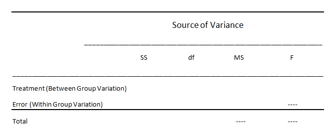
What we have to do now, is fill in these empty spaces. for this example, we will introduce the formulas as we work through the problem.
Step 1: find
Step 3: find (Between-group variation)
Step 3: find (within-group variation)


Step 4: Degrees of Freedom
Step 5: Calculate Mean Squares
Step 6: Calculate F ratio
Step 7: Complete the summary ANOVA table
.PNG)
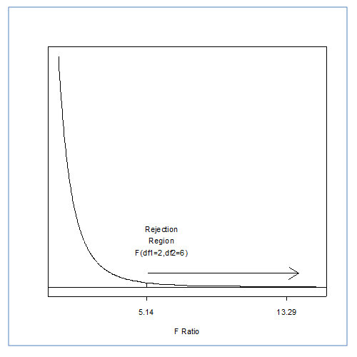
The end point of the summary ANOVA table is the F ratio. Now we can move on to the decision. Is there a difference in reaction times between the levels of alcohol consumption?
Step 8: Compare to the critical F ratio
For our decision, we will use the same concept that we have used to this point. Does our calculated F ratio pass the critical F ratio? There are, of course, a few differences to understand. With the t test, our critical ratio was based on the alpha level as well as our df. The same holds true for the ANOVA, but now we have two df's. Which one do we use? Well, we will use both!
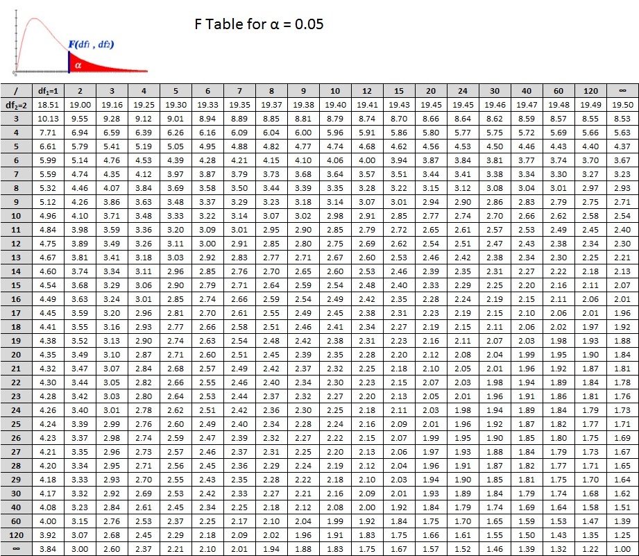
In the tables below, you see that the critical values are based on  . We can translate this into
  or F(2, 6). So for our example we read down the column for
  and across from the row for
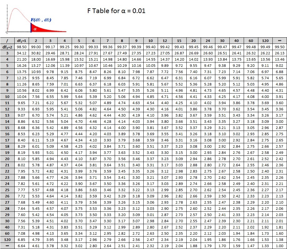
  . Don't forget the alpha level! There are 2 tables, one for 0.05 and the other for 0.01. Let's use Alpha = 0.05. What's the critical F ratio?
So what's your decision?
PRACTICE PROBLEM 9
Four groups of subjects were randomly selected from a population of high school seniors and were each subjected to different experimental educational programs. The subjects were then evaluated based on a 20 point scale, the subject scores were:
| Group 1 | Group 2 | Group 3 | Group 4 |
| 5 | 7 | 8 | 15 |
| 4 | 5 | 7 | 14 |
| 3 | 6 | 6 | 18 |
| 6 | 8 | 8 | 12 |
Did any of the selected groups respond differently to the treatments? Test the null hypothesis that there is no difference.