Hypothesis Testing with the Z score
We can compare our calculated Z scores to these critical values in order to make a decision. We will use the same Z score formula to accomplish this with a slight concept modification due to sampling error. Before we were just taking a simple score from a population of scores and converting it to a Z score.
To conduct a hypothesis test we will compare our sample to the theoretical distribution described by the null hypothesis (the hypothesis of "no difference" or "no effect"). To accomplish this, we need to describe a theoretical idea called the sampling distribution. Let's say that we have 10,000 people in our population. We want to measure the effects of our new wonder IQ drug. Our hypothesis is that it will INCREASE IQ. What type of hypothesis was this?(ANSWER) We can't test all 10,000, but we can take 100 and test them, then find their Mean. To be more accurate, we are going to do this again with another 100, and then another 100, and so on. If we were to take all these means, we have created a sampling distribution. This is where sampling error comes in. The more samples we take, the more the mean of our sampling distribution will look like the population mean. Each separate sample mean, however, will vary from the population mean. Sound a bit like standard deviation doesn't it? In fact, it is very similar and this is our modification. We are going to replace Standard Deviation with the standard deviation of the sampling distribution.
Z Score and the Standard Deviation of the Sampling Distribution:  (based on the population's SD)
When we first saw the Z score we were determining where a single observation fell compared to the mean of a normal distribution. Now we want to know where the mean of an entire sample of observations falls with regards to the mean of the sampling distribution. The basic concept of the Z score is the same - only some of the details are different.
The standard deviation of the sampling distribution is found with the formula:

Note that the numerator σ is the standard deviation of the population our sample is drawn from. Unfortunately, in practice we almost never know the value of this. Like we saw with confidence intervals when we don't know the population standard deviation we have to estimate from our sample which leads to a modification in our procedures. We'll cover that soon.
So, the Z score for our sample mean is found with the formula:

Note that the difference between this formula and the Z score formula we first saw is that now we are addressing the position of a sample mean compared to a population mean in the sampling distribution, rather than an individual value to the population mean of the individual observations.
All that is left for us to do, is the hypothesis test. Let's work through one using the following example.
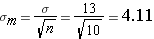
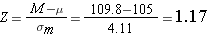
Let's say that the IQ test of a certain population has a M=105 and a σ=13. We hypothesize that our newly developed wonder drug will boost the IQ scores of all individuals who take it. To test this we sample 10 individuals from this known population and find the following IQ scores after they receive the treatment:
| 105 | 108 | 110 | 115 | 104 | 103 | 125 | 109 | 112 | 107 |
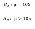
Remember that the null hypothesis is a statement of "no effect" so this null hypothesis states that the wonder drug has no effect on IQ scores ("innocent until proven guilty"). The alternative (research) hypothesis is the statement that the wonder drug does boost IQ scores.
Lets do this step by step:
Step 1: find the mean

Step 2: fin the standard deviation of the mean (using the population SD)
Step 3: find the Z score
Step 4: compare to the critical Z score
From the stated hypothesis, we know that we are dealing with a 1-tailed hypothesis test. Unless otherwise stated, we can assume an alpha level of 0.05. This gives us a critical Z score of: 1.64
Now we must decide whether to reject the Null hypothesis or fail to reject the null hypothesis. For this we always want to draw the distribution described by the null hypothesis so we can see where our sample is with respect to the null hypothesized distribution of "no effect."
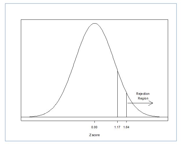
Remember that for something to be considered significant (leading us to reject null hypothesis) then the calculated Z score must be farther away from the mean than the critical value. We call the area past the critical value the rejection region. If any calculated ratio lands here, we reject the null hypothesis because our value is significantly different from the population. If it were to land before the critical value, we would fail to reject the null. In this case, because our sample mean is closer to the mean than the critical value, the correct decision is to fail to reject the null hypothesis. Our sample was not significantly different from the null hypothesized population of "no effect" due to the new wonder drug. In other words, the modest increase in IQ scores could be explained by chance variation and not necessarily due to the wonder drug.
Let's look at an example using a 2-tailed hypothesis.
Actually, let's just change the last example (to save us all a little work). This time, let's say that we THINK that the wonder drug will alter our IQ. We just don't know if there will be an increase or a decrease (which would be unfortunate). We will work with the same population with a μ=105 and a σ=13 and the same sample of 10 individuals:
105, 108, 110, 115, 104, 103, 125, 109, 112, 107
Review the above steps 1-3 because they would of course be the same. Step 4 will change a bit. This is where we make our decision.
Step 4 : compare to the critical Z score
We know that we have a 2-tailed hypothesis and we are working with an alpha level of 0.05. Now, however, we have a critical Z score of +/-1.96. To make our decision we will again draw a distribution.
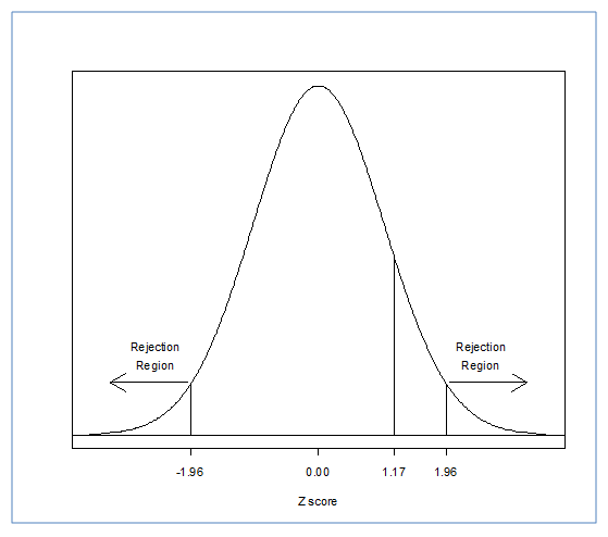
For the 2-tailed hypothesis test, the calculated z score must still be farther away from the mean than the critical value. The difference is that the alpha level was split across both tails giving us 2 critical values. So, we consequently have 2 rejection regions with the area in between representing the population. Note that for the same 0.05 alpha level the two-tailed test places the rejection region farther away from the mean than for the one-tailed test. For this reason you must think carefully about whether to use a one-tailed or two-tailed test as you could come to opposite conclusions with the same data depending on which kind of test you carry out. Chose a one-sided test if you suspect the effect is in only one direction – otherwise choose a two-sided test. In this situation, we still fail to reject the null hypothesis. Our sample mean still does not differ significantly from what we might expect if the null hypothesis of "no effect" is true. Note that failing to reject the null hypothesis does not mean we can say the null is true. It could be the wonder drug does have a small effect on IQ, but one that is too small for us to detect with this test. All we can conclude is that the sample IQ mean is consistent with what we would expect if the drug had no effect.
PRACTICE PROBLEM 6
A population of adult males has a mean weight of 175 pounds with a standard deviation of 25 pounds. A researcher wants to know if the mean weight of males in a particular area is different from the population mean. A random sample of 20 males provided a sample mean of 188 pounds. Carry out a hypothesis test to determine if this is evidence of a significant difference for the mean weight of adult males in this area.