t ratio
Now that we have the concept of hypothesis testing down, we will see that the concept does not change though the situation of the test might. For example, for the previous tests using the Z score we had detailed knowledge of the population. Namely, we knew the mean and the standard deviation of the population.
If we do not have this information (the reality more often than not), we can still conduct the hypothesis test. This brings us to the next analysis, the t test. The t test exists in multiple forms. In this module, we will be concerned with the one-sample t test, and the two-sample independent t test.
One-sample t test
The one-sample t test is not very different from the Z test with the minor exception that we do not know the population's variance. We are still comparing our sample to the population. But the lack of knowledge of the population variance means that we have to estimate the standard deviation. If we randomly sample from the population then our estimate should reflect the populations variance. However, the estimate will always be an underestimation of the true population variance.To account for this underestimation of the true population variance, we employ the t distribution. The t distribution resembles the normal distribution in that it is a symmetric and bell-shaped distribution. There are two important differences, however. First, the t –distribution is actually not a single distribution, but rather a family of similar distributions, each one characterized by a different value called the degrees of freedom. Degrees of freedom (df) is the number of independent pieces of information that go into the estimate of a parameter – typically the number of pieces of data minus the number of parameters used to produce the estimate. Since variance is calculated using a single parameter (the mean), the number of degrees of freedom for the one-sample t test is n – 1. The second important difference is in the tails of the t distributions compared to the normal distribution – basically they reach out farther. This greater width allows for a little more "wiggle room" for having to produce an estimate for the population variance (recall that the square root of variance is standard deviation).
This is where we will use the sample standard deviation S as our best estimate for the population standard deviation σ. Recall the computational formula for the sample standard devation.

Now, when it comes to the hypothesis test we have much the same issues as with the Z score hypothesis test. We have to distinguish between one-tail and two-tailed hypothesis, and we also need to account for sampling error. But of course, the standard error of the mean will be a little bit different.
Standard error of the mean:  (based on the estimated standard deviation)
Since the t distribution is based on sample scores, we will be using  as our measure of standard deviation (as opposed to
  or SD which would be based on the known population's standard deviation, refer back to Standard Deviation in module one) because our population parameters are unknown and we are forced to estimate them.

t ratio
Another difference; now we are calculating the t ratio rather than the Z score. If you look closely, however, you will see that there isn't a lot of difference.

The only thing left is the hypothesis test.
A professor is interested in a new studying method, but is unsure whether it is effective. His typical class final exam average is a 75. The professor takes a random selection of 20 students and teaches them the new study method. On the next final, the sample of students scored as follows:
| 95 | 90 | 80 | 70 | 60 | 94 | 88 | 70 | 63 | 69 |
| 88 | 87 | 91 | 75 | 78 | 80 | 66 | 55 | 91 | 73 |

Again, lets go through this step by step:
Step 1: find the mean

Step 2: find S
Step 3: find the standard error of the mean (using S)

Step 4: find the t ratio (for the one-sample t test)

Step 5: compare to the critical t ratio
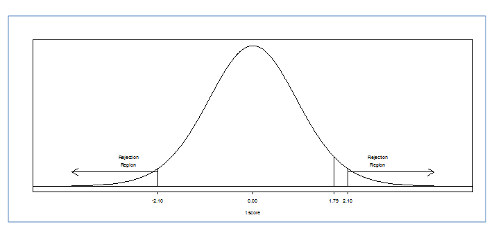
From the stated hypothesis, we know that we are dealing with a one-tailed hypothesis test. Unless otherwise stated, we always assume an alpha level of 0.05. Again deviating from the Z score, we no longer have constants. Now we must go to a table of critical t ratios like the one shown below in this T - Distribution table.
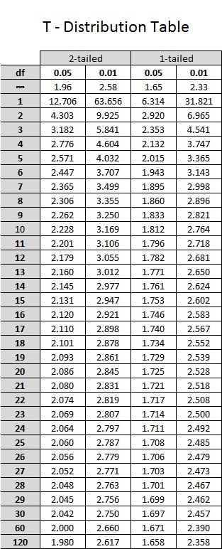
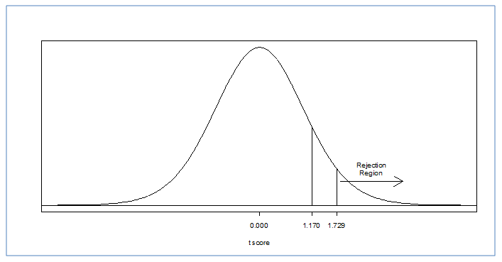
Since we are estimating population parameters, we can no longer base our results on the normal distribution. But, as stated before, the larger the sample, the closer to the population (and the normal distribution) that we come. In fact if you look at the first row in the table you will see that with an infinite number of subjects, our critical values are identical to those of the normal distribution (the critical Z's). However, since we are never going to work with an infinite data set, we must stick with our degrees of freedom to describe our distribution. For a one-sample t test, with a one-tailed hypothesis test, at an alpha = 0.05 and a df = 19; we get a critical t ratio of 1.729. So what is our decision? I advise everyone to continue to draw out your distribution, just like you did with the Z scores. Now, instead of a critical Z score, we have a critical t score, but the concept remains the same. Does our t ratio of 1.17 pass our critical value of 1.729? No. Therefore we fail to reject the null hypothesis. This means we do not have enough evidence to claim the professor's new study method is effective. Note that we can't conclude the study method is not effective – we can only conclude our sample results are consistent with what we would expect if the method was not effective. It could be the method does benefit students somewhat, but our hypothesis test cannot detect such a small difference if it does exist.
What if this had been a two-tailed hypothesis test at an alpha level of 0.01? Would we have made the same decision? ANSWER
What about a two-tailed hypothesis test at alpha = 0.01? ANSWER
PRACTICE PROBLEM 7
A random sample of seven college sophomores was selected and the students were tested for their attitudes toward gun control (high scores indicate a pro attitude and low scores an anti attitude). Their scores were 20, 18, 15, 11, 11, 8, 4. Test whether these sample scores deviate significantly from a known value of 18.00.
Two-sample Independent t test
Now instead of comparing a sample to the population it was taken from, we will compare two samples that are independent of one another. Our goal will be to determine whether the means of the two independent populations from which the samples are drawn are significantly different.
This could mean that we are comparing one sample that could be a control group (the group with no treatment or the standard treatment that serves as a basis for comparison) to another sample that could be a group that we gave a new medication to. If they are not significantly different (fail to reject null; they are consistent with the hypothesis of being from the same population) that would mean that our drug had no effect. We may also just be comparing two different classes taking the same exam. Are these groups different for some reason or do they represent the same population?
The steps for this are much like the previous, but with a couple of small changes.
The first change concerns the standard error of the difference in the means of the two populations. Once again we won't know the population standard deviations (neither of them), so we will have to use the sample standard deviations to stand in their places, thus leading to the use of a t distribution. But our parameter of interest is the difference in the two population means, so we need to calculate the standard error of this difference. The formula for this standard error is:
Estimated Standard Error of Difference:
(Note – You might have observed a slight inconsistency in the choice of symbols for this particular standard error – referring to it as SED rather than SD. The truth is -- either is fine. Statisticians do not have a single universally adopted notation system. Other variations you could run into are  .
.
The null hypothesis will be  reflecting the "innocent until proven guilty" notion of "no difference between the means of the two populations. Note that some people will write the null hypothesis as
  which is just a simple algebraic rearrangement of the first version. It makes no difference which population is identified with the subscript of 1 and 2 and is simply a matter of convenience. Subtract one way and the difference is positive. Subtract the other way and the difference is negative. Either way will lead to a t score that is either in or not in the rejection region of the null hypothesized t distribution.
The alternative hypothesis is also written about the difference of the two means and can either be one-sided ( ) or two-sided (
 ) depending on the researcher's question of interest.
The final difference has to do with the calculation of the t test statistic. It is the same as before in basic concept, but with a few details modified for our interest being in a difference of means:
Since the null hypothesized difference in means will generally be zero, you will also see this formula written as:
Or sometimes as:
While this last version is technically correct, it does tend to somewhat disguise the general form of a hypothesis test statistic (look back at the one-sample t or one-sample z for comparison). No matter how you write it, the t statistic will have degrees of freedom roughly as  (note that much better, but more complicated, estimates of the degrees of freedom are available with statistical software).
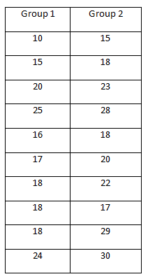
Lets go through another example, step by step. You run a test prep service and are reviewing the ACT scores of 2 different test groups to see is one of the groups responded to the service differently from the other group. Each group consisted of 10 testers and their scores were as follows:
Is this a directional (1-tailed) or non-directional (2-tailed) hypothesis?

where  is the mean of population 1 and
  is the mean of population 2.
Step 1: find the mean of each sample
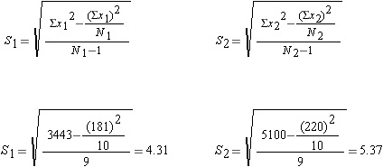
Step 2: find the standard deviation of each sample
Step 3 : find the standard error of the difference
Step 4: find the t ratio (for the two-sample independent t test)
Step 6: compare to the critical t ratio
For our decision, we are going to use the same T - Distribution table we used for the one-sample t test. The only thing that changed is the degrees of freedom. For the one-sample t test we used df=N-1. One sample; one N. For the two-sample independent t test, we have two samples; therefore, two N's. The df for the two-sample independent t test is equal to:
So for our case,
So we look for the critical t ratio in the table using alpha = 0.05, df = 18, for a two-tailed hypothesis. Is this significant? Do the samples represent one population? Do we reject the null hypothesis? ANSWER
What if we had made the hypothesis that group two would perform better than group one? ANSWER
PRACTICE PROBLEM 8
A researcher wonders if students will spend more time studying for a quiz if they are told that a high mark on that quiz will excuse them from writing a term paper. Two groups of college students were randomly selected from a large lecture course in art history. The students in Group 1 were simply told that they would have their first art-history quiz two days later. In Group 2, they were told the same thing, except that the promise of "no term paper" for high quiz performance was added. Just before taking the quiz, all students in both groups reported (in hours) the time they had spent preparing. In Group 1, the times were 6, 4, 9, 3, 2, 5, 7, 4, 7, 6. In Group 2 the times were 12, 5, 13, 5, 5, 7, 9, 6, 9, 6. Do you reject or fail to reject the null hypothesis?