Z scores
We have spent some time going through the concepts of hypothesis testing. Now let's look at how we can perform a hypothesis test, first, by using the Z score. We will start with an understanding of Z scores.
A Z score is a number of standard deviations a score is above or below the mean. In the Standard Normal Distribution, the mean is always equal to 0 and the standard deviation is equal to 1.0. The Z scores help us to describe various aspects of the distribution, such as percentile ranks, percentages of scores between points, etc. In short, it allows us to compare any one score to any other score in a distribution, or across distributions because it is standardized based on the distributions mean and standard deviation. Take a look at the following diagrams of the normal distribution. This breaks down the percentage of the distribution falling between the Z scores. This is a constant. Thus we can see that almost, but not quite all of the distribution lies between the Z scores of -3 and 3.
Normal distribution and Z scores:
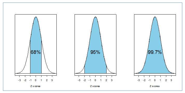
This 3-part diagram shows the percent of a normal distribution that lies between 1, 2, and 3 standard deviations from the mean: between -1 and 1 you can find approximately 68%; between -2 and 2 is approximately 95%; and between -3 and 3 is approximately 99.7% -- practically everything! All normal models follow this pattern, so a common name for this property is the 68-95-99.7 Rule. These percentages also represent the probability of finding a z score in one of these intervals, so this rule can be useful in answering probability questions such as we find in hypothesis testing.
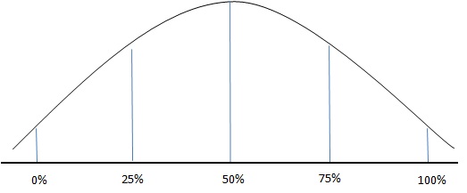
Here is another view of the Standard Normal Distribution. In this diagram the percentages represent the amount of the distribution between consecutive Z scores (-2 and -1, -1 and 0, etc.).
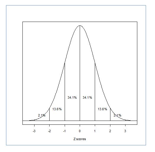
The diagram also illustrates how the Z scores fall on the normal distribution. Each Z score represents a unit of standard deviation away from the mean. To understand this lets look at an IQ distribution with M=100 and SD=12. A Z score of 1 is 12 units away from the mean; a Z score of 2 is 24 units away from the mean and so on. Because the normal distribution is symmetrical about the mean, as you can see by the percentage breakdown, then a Z score of -2 is also 24 units away from the mean.
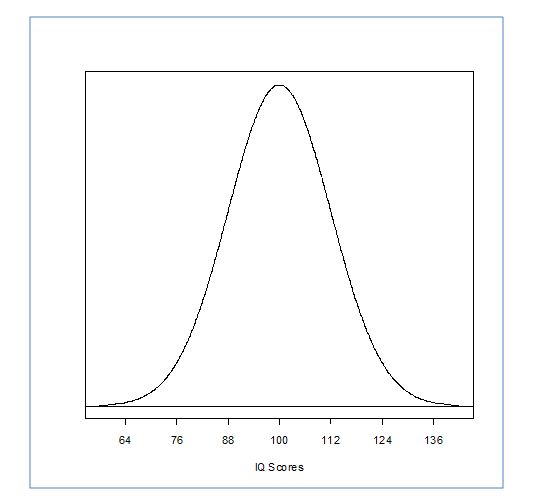
Now let's look at this in terms of raw scores. If the mean of our distribution is 100, then a Z score of 2 is equal to a raw score of 124. A Z score of -2 is equal to a raw score of 76.
Now we can start to compare individual's scores on this test. A problem we might run into however, is that our raw scores (the scores individuals get on the IQ test) will rarely fall right onto our Z scores. So we will have to know how to convert each raw score into a Z score. And vice-versa, we will need to know how to convert our Z scores into raw scores.
So, what if our friend Carl was one of the individuals in this distribution of IQ scores. He scored a 115 on the test. What is his Z score? Following the information already given, we know that a Z score of 1 is equal to 112 and a Z score of 2 is equal to 124. Therefore we know that Carl's Z score should be between 1 and 2. But to find out the exact Z score we turn to the Z score formula:
![]()
Thus:
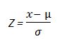
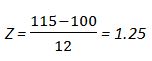
If Carl scored 115 of the IQ test, his converted Z score is 1.25. This means Carl's IQ is 1.25 standard deviations above the population mean IQ score. Why is this important? Well lets say that our cousin Bob just took the IQ test in another location (part of a different distribution). The mean of that distribution was 105 with a standard deviation equal to 18. Who performed better? We can't just compare them directly because the distributions are different. Hence the standardization of our scores. If Bob scored 118 let's find his Z score.
![]()
So even though Bob's raw score was higher, after standardization,we can conclude that Carl scored higher relative to others in his distribution than did Bob.
Let's go the other way now. Going back to our first distribution (M=100, SD=12) we know that another individual had a Z score equal to -0.95. We can find this by solving the Z score formula for x.
.JPG)
This demonstrates that we can use Z scores to gain understanding into an individual's performance. We can also use them to determine where in a distribution a scores falls. To accomplish this we will turn to the following table.
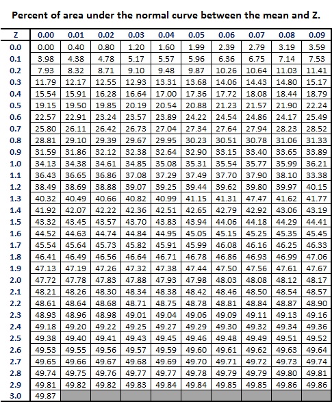
As the title of this table suggests, we can use Z scores to determine how much of a distribution is represented. This particular Z score table, and there are many versions, only gives the area under the normal curve for points between the mean and Z as depicted below.
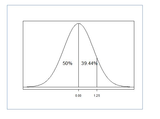
So, If we have a Z score of 1.25 then the area under the curve from Mean to Z is 39.44%. But remember that we still have the other half of the distribution. Since a normal distribution is symmetrical, that means that 50% lies on both sides of the distribution. So, if we have a Z score of 1.25, that means that it is at the 89.44th percentile (39.44+50). It also means that even though the information is not given, we know that 10.56% is in the area beyond our Z score.
PRACTICE PROBLEM #1
What percentage of scores would fall below a Z score of 2.56?
PRACTICE PROBLEM #2
What percentage of scores would be greater than a Z score of -1.56?
PRACTICE PROBLEM #3
What percentage of scores would fall BETWEEN Z scores of -1.0 and 1.0?
Now let's go backwards from a percentage to the Z score. What if we know that a particular score is at the 85th percentile? Using the Z score table, what could we use as the Z score? The Z score would be 1.03. What if we knew that exactly 2.5% of the distribution was beyond our Z score? What is that Z score? 1.96. (we will see this one again). HINT: remember to draw the distribution. Percentiles range from the 1st percentile towards the 100th percentile
If you didn't guess these, remember that we have to account for the 50% of the distribution in the other half, and that our table only gives us from the mean to Z. So for 85%, we have to subtract 50 to get 35%. We then look for the value closest to 35% (or the value just below it) and move backwards to find our Z score. 1.03, see? For 2.5%, we have to remember that we are looking at the area beyond the Z, therefore we must subtract it from 50. 50 - 2.5= 47.5. Giving us a Z score of 1.96.
PRACTICE PROBLEM 4
What is the Z score for the 15th percentile ?
PRACTICE PROBLEM 5
What is the Z score for the 75th percentile?
You may have asked yourself (several times, in fact) why this matters, or of what use is this information? Well this is how we are going to determine if there is a significant difference between groups. We will do this by setting a critical value, a threshold, using the alpha level and corresponding Z scores in much the same way that we have been practicing. This critical value is going to look at the area beyond the Z score as this will represent the scores that ARE NOT in the typical population.
Of course, this is going to require some additional knowledge; the difference between a 1-tailed hypothesis and a 2-tailed hypothesis. A 1-tailed hypothesis means that we, the researchers, are predicting a specific response. Putting it into our Magistrate example, if we were to predict a DECREASE in the number of deaths after eating citron then we just stated a 1-tailed hypothesis. If we were testing a new pill that changed our IQ, we could make another 1-tailed hypothesis by stating that the drug would INCREASE our IQ. The 1-tailed hypothesis is directional. A 2-tailed hypothesis on the other hand means that we had no specific idea of what would happen. For example, we could be engaging in exploratory research to discover whether our new teaching method increased OR decreased the average performance in our classroom. The 2-tailed hypothesis is non directional.
Let's tie this together by first looking at a scenario using an alpha level of 0.05. If you look at the normal distribution diagram, you see that 0.05% would be in the tails. So conversely 95% of our distribution would be in the main body of the distribution. If we have a 2-tailed hypothesis test, that means that we have to split this 5% among both tails. So for a 2-tailed hypothesis test, if the alpha level is set at 0.05, then moving backwards from 2.5% (the area under the curve, beyond the Z) to a Z score we get +/-1.96. Since it is 2-tailed, we don't know if our score will be on the high or low end of the distribution hence the positive or negative Z score. In any case, this is our critical value. In this case a critical Z score. This means that the probability of an event occurring by chance, using the normal distribution, is 5%. We need our calculated Z score to pass 1.96 (the critical value) to be significantly different than the rest of the population at a level greater than chance.
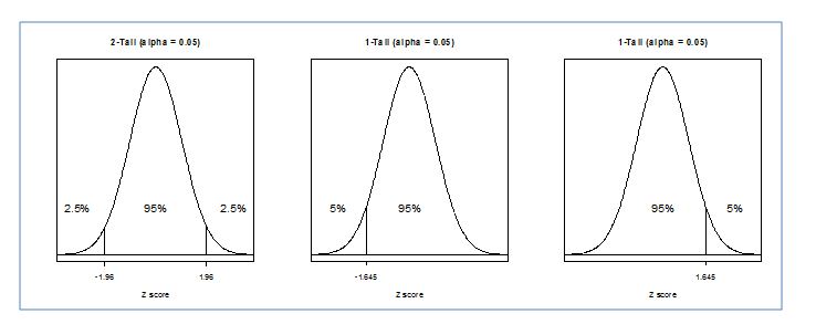
What if we set the alpha level at 0.01? For a 2-tailed hypothesis test, the z score is +/- 2.58. This should start to make intuitive sense. An alpha level of 0.01 is more conservative than one of 0.05 because we are now saying that there is only a 1% chance of committing Type I error. 2.58 is larger than 1.96, therefore it is more difficult to show significant difference at the 0.01 level because our calculated Z score now has to pass the critical Z score of 2.58.
This of course, was looking at a 2-tailed hypothesis test. What about 1-tailed tests? We still need to find a Z score that corresponds to our alpha level, but now the entire percentage would lie in one tail, on one side of the distribution. An alpha level of 0.05 for a 1-tailed test would therefore be equal to a critical Z score of 1.64. An alpha level of 0.01 for a 1-tailed hypothesis would be equal to a critical Z score of 2.33.